Four questions before an algorithm decides about people
Abstract
Credit scoring is the oldest mass deployment of algorithms deciding about people, and the best place to learn what responsible AI means in practice. Four questions every team should be able to answer about its model — can we explain the decision, does it reason like our experts, are we fair, do the numbers mean what they say — and five steps to start on Monday. The figures run on a seeded synthetic credit portfolio; code included.
“Why did you turn me down?” The question comes from a bank customer, a job candidate, a citizen at a benefits office. An organisation that runs on automated decisions should be able to answer it three ways at once: quickly — in a minute, not after a week of analysis; truthfully — according to what actually drove the decision; and consistently — the same way for every person. If it cannot, it is not the organisation making the decision. It is an algorithm nobody in the building understands.
I build credit‑risk models for Allegro Pay, a buy‑now‑pay‑later lender that makes millions of automated credit decisions. This note is the written version of my talk at Polski Kongres AI in Łódź, and it is aimed at anyone who lets a model decide about people, not only at lenders.
Credit scoring as a proving ground
Scoring is worth learning from because it has every property that makes algorithmic decisions hard: the decisions are automated, made at scale, matter for people’s lives, and have been supervised for decades. The questions transfer almost word for word:
| Area | The AI decides | The same question |
|---|---|---|
| Credit | approve? what limit? | can we explain it? |
| Insurance | what premium? | is the price fair? |
| HR and hiring | whom to interview? | are we discriminating? |
| Public administration | who gets a benefit, who gets audited? | can the citizen appeal? |
| Collections | whom, when, how? | do we treat people alike? |
Swap “credit” for your own decision; the rest of this note still applies.
The calendar is fixed, too. In Poland, supervision under the act on AI systems — by the new commission, KRiBSI — starts on 28 October 2026, the day of the talk. From 20 November 2026 the second Consumer Credit Directive (CCD2) gives borrowers the right to an explanation of their creditworthiness assessment and to a human review of the decision. From 2 December 2027 the AI Act’s obligations for high‑risk systems apply, and Annex III reaches far beyond credit: hiring, education, access to public services, insurance. The legal detail is for lawyers. What follows is the engineering practice that makes the law easy to comply with.
Four questions for your AI team
- Can we explain the decision? To the person, to the regulator, and to ourselves.
- Does the AI reason like our experts? Do its reasons make business sense?
- Are we fair? And who decides what that means?
- Are the numbers true? Today, and after the world changes.
None of them is a question about the algorithm. All four are questions about governance.
1. Can we explain the decision?
Modern models beat points tables on accuracy, but out of the box they are opaque. And an explanation is not one report — it is three different products for three audiences:
- The person needs a few understandable reasons and what could change the outcome. That is the right to an explanation in CCD2.
- The regulator and the auditor need to know how the model works, what it learned from, and how it is controlled. That is the AI Act’s documentation duty.
- We ourselves need to know the model has not learned nonsense and still behaves as it did on release day. That is quality control.
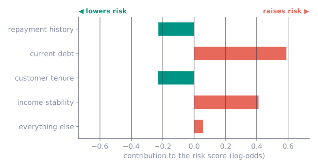
For the first audience, a model with hundreds of inputs cannot hand a person hundreds of attributions. We group the variables into domains a human understands — repayment history, current debt, tenure, income stability — and report the few that mattered: “Your current debt was decisive. Repaying part of it would improve your assessment.”
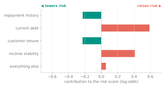
The catch is in the second sentence. An explanation has to be true, not merely tidy. Attribution methods such as SHAP divide up a score that already exists; they do not say what would happen if the customer acted on them, and on a real model the advice can point the wrong way. I took that failure apart in Why SHAP values are not points; the honest answer to “what would change the outcome” is a verified counterfactual, which is what treecf computes.
2. Does the AI reason like our experts?
Accuracy is not enough: a model can be right for the wrong reasons. Two checks catch most of it.
Check the directions. Does a better repayment history lower the risk? Does more debt raise it? Every direction that contradicts domain knowledge needs a written justification before the model reaches production. That is an acceptance criterion, not an optional extra.
Group people by their reasons. Two applicants with the same score can be there for entirely different reasons — one is new to credit, the other is overextended. Segmenting by why, not only by how much, produces better communication and better products. Explainability is not a compliance cost; it is knowledge about your customers you did not have before.
3. Are we treating people fairly?
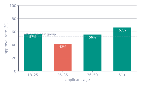
Groups differ in age, region and history, so model outcomes will differ too. A difference is not yet discrimination — but every difference needs an explanation. On the synthetic portfolio behind this note (60 000 applicants for training, 40 000 for evaluation, an 8.4% default rate, an XGBoost model approving below 8% predicted PD), approval rates differ markedly by age:
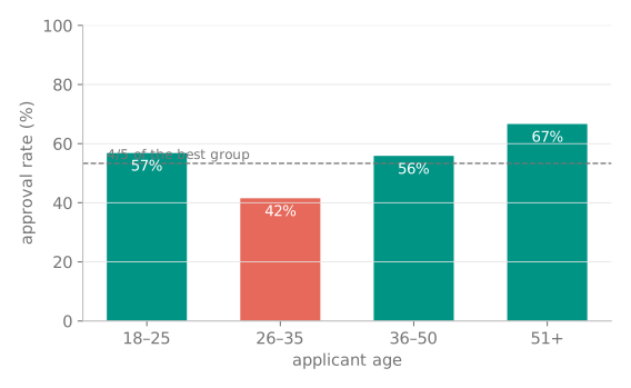
The four‑fifths rule is a warning line, not a verdict. What matters is the process around it: measure regularly, keep a threshold, and send every breach to a review that either explains the gap with legitimate risk factors or changes the model.
Ask who applies before you blame the model. The first thing the review should check is whether the gap comes from the model at all. A lender never sees an age group; it sees the part of that age group that chose to apply, and the choice is rarely random. In the simulation, financial strain drives applications at every age, but far more strongly among the young: a 23‑year‑old with savings seldom needs to defer a payment, so the young people who do apply are disproportionately those already stretched. The model is the same in every comparison below; only the people it is applied to change:
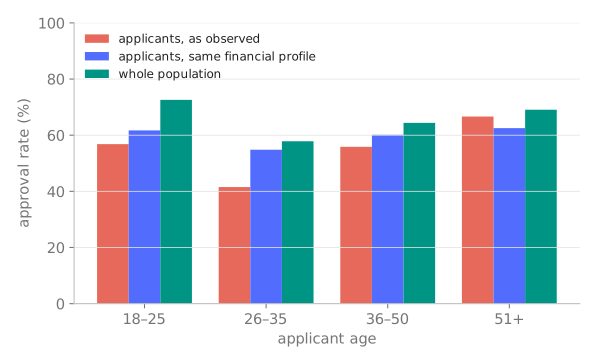
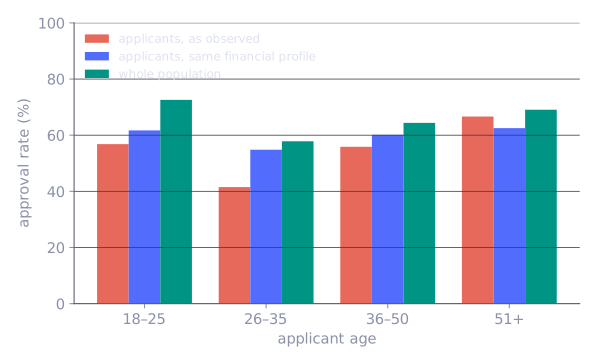
The whole population is rarely available, but the “aligned” comparison is something any team can run on its own data. Train a classifier to predict the group from the risk‑relevant features — here utilization, delinquency, active loans and income stability, deliberately without age or tenure — and weight each applicant by P(group) / P(group | x). Every group then has the same financial mix, and whatever gap survives is the model treating similar people differently. That residual is what needs a justification. The rest is a question for product and marketing — whom does our offer attract, and why — not for the model. Selection cuts both ways, too: a gap that disappears among applicants can hide a population that never applies because it expects to be turned down.
Removing the sensitive attribute does not remove it. The model behind this note never sees sex. It does see shopping behaviour: the main purchase channel, the share of automotive purchases, the time of day someone shops online. None of them carries risk of its own in the simulation; each correlates with sex. Train a classifier to recover sex from them and it gets there easily:
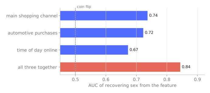
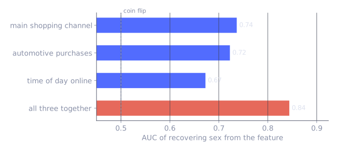
This is how real systems have gone wrong — a recruiting algorithm that learned to penalise CVs mentioning women’s organisations, public‑sector fraud‑detection systems that ended in scandal. And the simulation adds a twist worth remembering: dropping the three proxies does not close the gap either. Approval is 63.3% for one sex and 59.0% for the other with the proxies, 63.2% and 58.7% without them, because here the gap flows through income stability, a legitimate risk driver that also correlates with sex. Deleting columns is not a fairness strategy. Measuring outcomes by group is.
Fairness has a measurable price. All definitions of fairness cannot be satisfied at once — outside trivial cases it is a theorem (Kleinberg, Mullainathan & Raghavan, 2016). So the choice is one of values, and the honest thing a data team can do is put a price on each option. In the simulation, each approved good loan earns one unit and each approved default loses the amount that makes the 8% cutoff break‑even. Lifting the lower‑approval age bands with their next‑safest applicants traces the trade‑off:
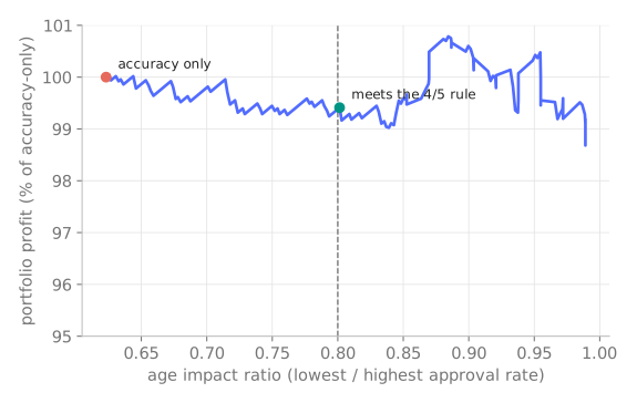
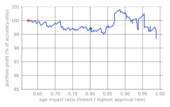
Here the price is small, and that is no accident: the applicants it takes to close the gap are the next‑safest in their band, sitting just above the cutoff, where a loan barely loses money. On another portfolio the curve can fall steeply. Either way the number has to be measured, not assumed, and where to stand on the curve is a decision for the board, not for the algorithm.
What works in practice: measure outcomes by group even when the attribute is not in the model; separate the applicant mix from the model’s own treatment; track several measures at once — access, errors, accuracy; and run a fundamental‑rights impact assessment (FRIA) before deployment. A model can also discriminate through how confident it is rather than through what it decides — I wrote about that in Discriminatory uncertainty.
4. Do the numbers mean what they say?
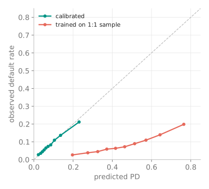
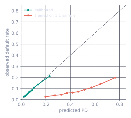
Prices, budgets, queue priorities and resource allocation are built on the probabilities a model outputs. If a probability is inflated or deflated, the decision built on it is wrong. The test is the one we apply to weather forecasts: when the model says 70%, the event should happen roughly seven times in ten.
A model can rank cases well and still get the values badly wrong. A common shortcut shows it: train on a 1:1 resample because the data are “imbalanced”, and never correct back. Same features, same algorithm; the ranking barely moves — AUC 0.677 against 0.684 — but the average predicted PD is 45.4% for a portfolio that defaults 8.4% of the time:
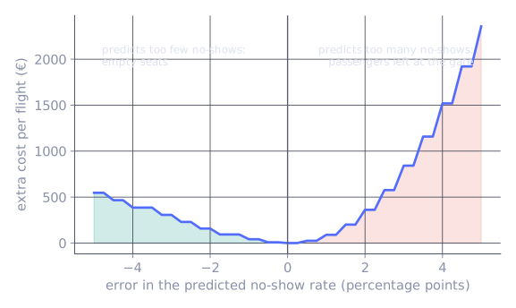
Errors in one direction can cost far more than in the other. Calibration matters most when the cost of being wrong is lopsided, and outside credit that is the normal case. Take airline overbooking. A 180‑seat flight, a true no‑show rate of 10%, and an airline that sells exactly as many tickets as minimises expected cost under the rate its model predicts. An empty seat loses a fare margin, say €90. A passenger denied boarding costs compensation — €400 under EU 261 on a medium‑haul flight — plus rebooking and goodwill, say €600 in all. Get the no‑show rate wrong by the same three percentage points in either direction:
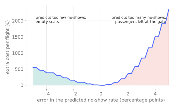
The same shape shows up wherever a probability drives an action: a sepsis alert in a hospital, where a missed case can be fatal and a false alarm costs a nurse’s time; stock in a pharmacy, where an empty shelf and an expired box are priced very differently. The decision threshold follows directly from the two costs — act when p > cost(false alarm) / (cost(false alarm) + cost(miss)) — but only if p means what it says. A well‑ranked, badly calibrated model puts the threshold in the wrong place, and the asymmetry decides how much that hurts.
Check both, ranking and values, every time. Calibration is the part of credit modelling I care about most; probcal is the library I wrote for it.
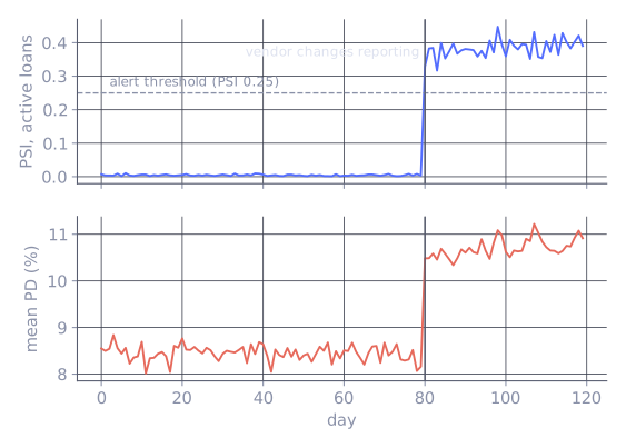
Responsibility does not end on deployment day. A real pattern, reproduced in the simulation: an external data vendor changes how it reports a field — here, it starts counting closed‑but‑not‑yet‑deregistered loans as active. Nothing about the applicants changes. The model runs flawlessly. And its scores shift overnight:
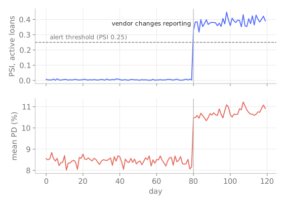
The defence is boring and effective: daily monitoring of inputs and outputs, alert thresholds with a defined escalation path, and a post‑mortem after every incident.
How to organise it
Model governance in practice rests on four things:
- An owner. Every model has a person accountable for it.
- Approval. A clear path from the expert team up to the board.
- Documentation. How the model was built, how it works, and what changed in it.
- Review. Regular, with explicit triggers for a rebuild.
The impact assessment before deployment is not a formality. Its conclusions can and should change the business plan.
Compliance as a by‑product of good engineering. The last‑minute version is documents written for the audit that drift away from reality — expensive, brittle and useless to the team. The built‑in version is documentation versioned with the model and reviewed like code, and every decision logged with the model version that made it. The test is an auditor’s question: “Why did this person get this decision fourteen months ago?” It should take minutes to answer, not weeks.
Where to start: five steps
- Inventory. Where does AI decide about people in your organisation, and who owns each system?
- The “why” test. Pick a random decision and ask for an explanation a layperson would understand.
- Measure by group. Age, sex, region — even if none of them is a model input.
- Calibration and monitoring. Do the model’s numbers match reality, every month?
- Board decisions in writing. Which trade‑off between accuracy and fairness do we accept?
None of these steps needs new technology. Each needs a decision. Trust scales; distrust costs.
Reproduce the figures
Every figure on this page comes from one seeded script — a synthetic population and the applicants who self‑select from it, an XGBoost PD model, an overbooking cost model, matplotlib: rai_gen_figs.py. Numbers in the text are its output, not illustrations. The data are synthetic and say nothing about any real lender’s portfolio.
This note is the written version of my Polski Kongres AI 2026 talk in Łódź, Odpowiedzialne AI w scoringu kredytowym (given in Polish). Slides: Odpowiedzialne AI w scoringu kredytowym (PDF) · all talks: github.com/wlazlod/conference-talks.
Cite this note (BibTeX)
@misc{wlazlo2026fourquestions,
  author       = {Wlaz{\l}o, Daniel},
  title        = {Four Questions Before an Algorithm Decides About People},
  year         = {2026},
  month        = oct,
  howpublished = {datadeer.pl},
  url          = {https://datadeer.pl/notes/four-questions-responsible-ai.html}
}